Imagine a 3000 km race across the Australian outback — Darwin to Adelaide along the Stuart Highway run almost entirely on sunlight. You get a few square metres of solar array, a battery pack small enough to fit in a Challenger-class car, and a clock that only counts between 08:00 and 17:00. Overnight the sun is gone; the pack is whatever you conserved. There are mandatory thirty-minute stops. First to Adelaide on legal time wins. That is the World Solar Challenge.

In a race like this, the car’s hardware sets the ceiling. Strategy decides how close you get to it. Given the vehicle you have and the irradiance you expect, how fast should you drive so that you arrive as soon as the energy budget allows — without emptying the pack? Drive too hard and you strand early; drive too conservatively and you gift hours to teams that spent the same joules better. The question is deceptively small. It is also the whole job.

I worked on that problem as race strategy engineer for Agnirath, the IIT Madras solar-car team, on Agneya, the Challenger-class car we took to the event representing India. This post is a brief on building a sufficient strategy model: the minimum-time formulation, the plant we integrate, why the solution collapses to one cruise speed per driving day, and a set of one-parameter tests that show which knobs actually move that speed.

On a hopeful plant the daily holds sit near 85 km/h; on the car we measured, near 76 km/h. A free spatial velocity profile did not improve on the daily hold. Irradiance and aerodynamic drag (including wind) dominate. Mass, at these speeds, does not.

---

Problem formulation

Objective

Formally, choose a speed plan $v(\cdot)$ and finish time $t_f$ to minimize time to Adelaide, subject to energy, the race clock, and the road:

\[\min_{v(\cdot),\, t_f}\; t_f \quad \text{subject to}\quad x(t_f) = X_f,\]

with $X_f \approx 3041$ km. The remainder of the model specifies how position $x$ and pack energy $S$ are allowed to evolve.

Plant

The equations below are what we integrate. Omissions are deliberate.

Kinematics. On the racing clock, $\dot{x} = v$. Acceleration is not treated as a continuous decision; start and stop are events. At cruise, $a = 0$.

Longitudinal force on grade $\theta(x)$ from the route data:

\[F = \tfrac{1}{2}\rho C_{DA}\, v^{2} + mg\, C_{rr}\cos\theta + mg\sin\theta.\]

Aerodynamic drag supplies the familiar $P \propto v^{3}$ term that dominates cruise. Rolling resistance is nearly constant in Wh/km. Grade is net climb; Stuart Highway slopes in our file are roughly $-0.6°$ to $+0.7°$.

Electrical power, with a single drivetrain efficiency and hotel load:

\[P_{\mathrm{mech}} = \max(Fv,\, 0), \qquad P_{\mathrm{elec}} = \frac{P_{\mathrm{mech}}}{\eta} + P_{\mathrm{aux}}.\]

We take $\eta = 0.92$ and $P_{\mathrm{aux}} = 50$ W as a baseline. The $\max(\cdot, 0)$ encodes no regeneration: downhill mechanical power is not returned to the pack. Motor thermal detail, loss maps, and chassis dynamics are folded into $\eta$ when needed (e.g. $\eta = 0.85$ as a hot-day sensitivity) rather than modelled as separate states.

Solar input follows the Gaussian irradiance model, scaled by array area and panel efficiency:

\[G(t) = A_p\, \eta_p\, I_0 \exp\!\left(-\frac{1}{2}\left(\frac{t-\mu}{\sigma}\right)^{2}\right),\]

with $A_p = 6$ m² and $\eta_p = 0.19$. The curve is bright relative to a conservative race week; that matters in the ablations below.

Wind is absent in the theory plant (still air). In later tests, airspeed is $v_{\mathrm{air}} = v - w_{\parallel}$ with $w_{\parallel} > 0$ a tailwind.

Battery as a watt-hour tank:

\[\dot{S} = G(t) - P_{\mathrm{elec}}, \qquad 0.2\, S_{\max} \le S(t) \le S_{\max}, \qquad S_{\max} = 3055\ \mathrm{Wh}.\]

Race constraints

These bind as tightly as the physics:

• Driving only in 08:00–17:00; outside that window $v = 0$, while solar and hotel continue (the latter, a pessimistic assumption).
• Thirty-minute parks at control stops (322, 588, 987, 1210, 1493, 1766, 2178, 2432, 2720 km - identified from the route).
• $0 \le v \le v_{\max}$ with $v_{\max} = 35$ m/s.
• Five legal days; $x < X_f$ at 17:00 on day 5 is a DNF (Did Not Finish).

That is the NLP. The rest is how I turn it into speeds I would actually radio.

---

Methodology

I did not invent the core idea. Classical solar-car optimal control — principally Howlett, Pudney and collaborators — already says that under standard models the optimum is a speed-holding (singular) regime, not a continuously wiggling $v(t)$ (Howlett et al., 1997; Pudney & Howlett, 1998; Pudney & Howlett, 2002). What follows is how that result sits on our plant and on the World Solar Challenge day structure, and the algorithm I used to turn it into five numbers.

Setup for a single driving window

Fix a driving interval $[t_a, t_b]$ (e.g. 08:00–17:00 on one day, excluding mandatory parks). On that interval assume:

1. Cruise kinematics: $a = 0$ almost everywhere while moving, so the control may be taken as speed $v(t) \in [0, v_{\max}]$ (start/stop treated as events).
2. Level or mild grade: resistive power admits the form \(\varphi(v) := v\, R(v) = \tfrac{1}{2}\rho C_{DA}\, v^{3} + mg C_{rr}\, v\) (plus a slowly varying grade term absorbed into $R$). In particular $\varphi$ is strictly convex and increasing on $[0, v_{\max}]$ because of the cubic aero term.
3. Electrical map: $P_{\mathrm{elec}}(v) = \varphi(v)/\eta + P_{\mathrm{aux}}$ with $\eta, P_{\mathrm{aux}}$ constant, so $P_{\mathrm{elec}}$ is likewise strictly convex.
4. Exogenous solar: $G(t)$ is a known function of time (irradiance forecast), independent of $v$.
5. Watt-hour battery with bounds: \(\dot{S} = G(t) - P_{\mathrm{elec}}(v),\qquad S_{\min} \le S(t) \le S_{\max},\) with $S_{\min} = 0.2\, S_{\max}$. Charge/discharge losses are neglected (ideal storage); under inefficient storage the literature replaces one hold by two critical speeds (Howlett et al., 1997; Pudney & Howlett, 2002). Our plant uses the ideal-tank case.

Energy consumed over the window and distance covered are

\[E[v] = \int_{t_a}^{t_b} P_{\mathrm{elec}}\bigl(v(t)\bigr)\, dt, \qquad X[v] = \int_{t_a}^{t_b} v(t)\, dt.\]

For a prescribed budget, feasibility requires that the induced pack trajectory stay in $[S_{\min}, S_{\max}]$ given $G$ and the overnight boundary conditions.

Theorem (constant speed, under the assumptions above)

The following is the classical speed-holding statement specialised to assumptions 1–5. It is not claimed as a theorem for the full World Solar Challenge plant with control stops, overnight clipping, and route grade from a file — only for the idealised driving window just defined.

Theorem 1 (constant-speed optimality on an idealised window). Under assumptions 1–5, among all measurable controls $v: [t_a,t_b] \to [0, v_{\max}]$ that attain a fixed distance $X_\star = X[v]$ with feasible pack trajectory, the unique energy-minimising control (when it exists in the interior) is the constant speed

\[v(t) \equiv \bar{v} := \frac{X_\star}{t_b - t_a} \qquad\text{for a.e. } t \in [t_a, t_b]\]

(ignoring measure-zero park sets). Equivalently, for a fixed energy budget, the distance-maximising cruise is constant at the largest $\bar{v}$ such that the constant-speed trajectory remains pack-feasible.

In particular, on that window the problem of covering as much highway as possible subject to the pack reduces to a one-dimensional search over a constant $\bar{v}$.

Proof sketch

(i) Convexity / Jensen. Strict convexity of $P_{\mathrm{elec}}$ implies, for any admissible $v$ with mean $\bar{v} = X[v]/(t_b-t_a)$,

\[\frac{1}{t_b-t_a}\int_{t_a}^{t_b} P_{\mathrm{elec}}\bigl(v(t)\bigr)\, dt \;\ge\; P_{\mathrm{elec}}(\bar{v}),\]

with equality iff $v \equiv \bar{v}$ a.e. Thus any non-constant profile that averages to $\bar{v}$ consumes strictly more electrical energy than holding $\bar{v}$. The same observation underlies the remark that a constant-speed strategy, where feasible, is essentially most efficient in energy terms (Pudney & Howlett, ANZIAM).

(ii) Optimal-control view. Writing the Hamiltonian for states $(x,S)$ with control $v$ and costates $(\lambda_x, \lambda_S)$, Pontryagin maximisation on a singular arc with efficient storage yields a speed-holding condition: $v$ is chosen so that the switching function vanishes on an interval, which for level-road models with convex $\varphi(v) = v R(v)$ forces $v$ constant (Howlett et al., 1997; survey in Betancur et al., 2017). Bang arcs (max power / regen) appear only at isolated junctions; they are not the bulk of a multi-hour cruise.

(iii) Minimum time $\leftrightarrow$ maximum distance. On a fixed clock window, maximising distance subject to energy is the operational form of “drive as far as the day allows.” By (i), any oscillation about a candidate $\bar{v}$ wastes energy that could have supported a higher constant speed. Hence the optimum, when interior and pack-feasible, is constant.

(iv) Remark on two critical speeds. If battery charge/discharge is inefficient, the singular condition splits into a lower hold (discharging while solar is weak) and an upper hold (charging while solar is strong) (Howlett et al., 1997; Pudney & Howlett, 2002). With a watt-hour tank and no storage loss, those two speeds coincide: one hold per window.

From the theorem to our race model (a working hypothesis)

Our simulator is richer than assumptions 1–5: $G(t)$ varies through the day, control stops force $v=0$ for thirty minutes at fixed kilometres, overnight recharge clips at $S_{\max}$, and $\theta(x)$ comes from a route file rather than a perfectly level road. So I do not treat Theorem 1 as a proof that Agneya’s optimum is five constants.

Why it is still a sensible hypothesis, approximately: cubic aero still dominates, so the Jensen penalty for oscillating about a mean remains the main energy argument; grades are mild enough that they belong in the integrator without justifying a free speed every few kilometres; and the race clock already chops the problem into days. Overnight, $\dot{S} = G - P_{\mathrm{aux}}$ with clipping at $S_{\max}$, so energy left at 17:00 that only refills to the ceiling by morning is hard to “save” productively — choosing the fastest feasible hold day by day is a natural greedy structure even if it is not proven optimal for the full multi-day NLP.

That suggests a working policy: daily cruises $(\bar{v}^{(1)},\ldots,\bar{v}^{(5)})$, constant within each driving day aside from mandatory parks. Whether this is good enough for our plant is empirical — checked after the algorithm.

Algorithm: daily cruise by bisection

For each morning state $(x_0, S_0)$ I compute the fastest constant speed that keeps $S(t) \ge S_{\min}$ until $t_b$ or until $x = X_f$. This implements the one-dimensional search suggested by the idealised theorem, on the full day simulator (stops, grade, time-varying $G$).

Algorithm 1 (DailyCruiseBisection)

Input: morning state $(x_0, S_0)$; day window $[t_a, t_b]$; plant $(P_{\mathrm{elec}}, G, \theta)$; bounds $[v_{\mathrm{lo}}, v_{\mathrm{hi}}]$ (e.g. $[0, v_{\max}]$); tolerance $\varepsilon_v$.

Output: cruise $\bar{v}^\star$ and simulated trajectory on that day.

1. Feasibility oracle. For a trial speed $v$, integrate \(\dot{x} = v,\qquad \dot{S} = G(t) - P_{\mathrm{elec}}\bigl(v, \theta(x)\bigr)\) on $[t_a, t_b]$, inserting 30-minute parks ($v=0$) at control-stop kilometre marks. Return true iff $S(t) \ge S_{\min}$ throughout and (if $x$ reaches $X_f$) the finish occurs with a feasible pack.
2. Bisection. While $v_{\mathrm{hi}} - v_{\mathrm{lo}} > \varepsilon_v$:
   • Set $v \leftarrow (v_{\mathrm{lo}} + v_{\mathrm{hi}})/2$.
   • If the oracle accepts $v$, set $v_{\mathrm{lo}} \leftarrow v$; else $v_{\mathrm{hi}} \leftarrow v$.
3. Return $\bar{v}^\star \leftarrow v_{\mathrm{lo}}$ (largest accepted speed) and its trajectory.
4. Overnight. From $t_b$ to the next $t_a$, integrate $\dot{S} = G - P_{\mathrm{aux}}$ with $v=0$, clip to $[S_{\min}, S_{\max}]$, and advance to the next day.

Monotonicity of the oracle in $v$ (higher cruise draws more power, so the feasible set is $[0, v^\star]$) makes bisection exact up to $\varepsilon_v$. The full race plan is Algorithm 1 applied sequentially for $d = 1,\ldots,5$.

Validating the hypothesis: daily holds vs a freer $v(x)$

If the classical constant-speed intuition were a bad fit to our plant, a freer spatial profile should find a meaningfully earlier Adelaide. To check that, I kept the same dynamics, stops, and clock, and compared:

• Piecewise daily cruise (Algorithm 1): one constant $v$ per driving day.
• Global-ish choice: 24 spatial bins (~127 km each), each with its own speed, searched with differential evolution and polished with L-BFGS-B. Objective: earliest clock time at Adelaide. Empty pack or a DNF scored worse than any legal finish.

The second is a real global search over a flexible $v(x)$, not a certified global minimum of the infinite-dimensional problem — but it is enough to stress-test the daily-hold hypothesis.

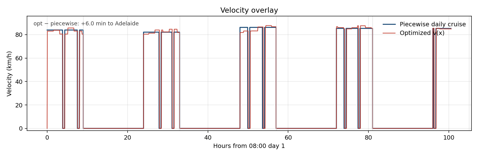
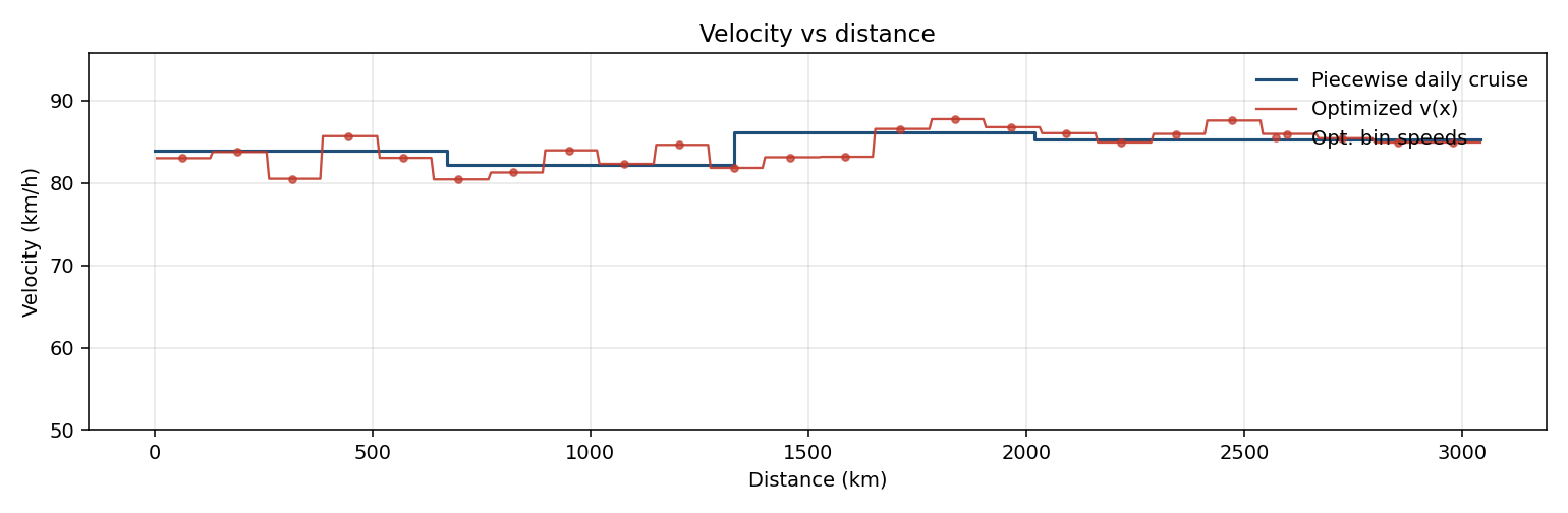
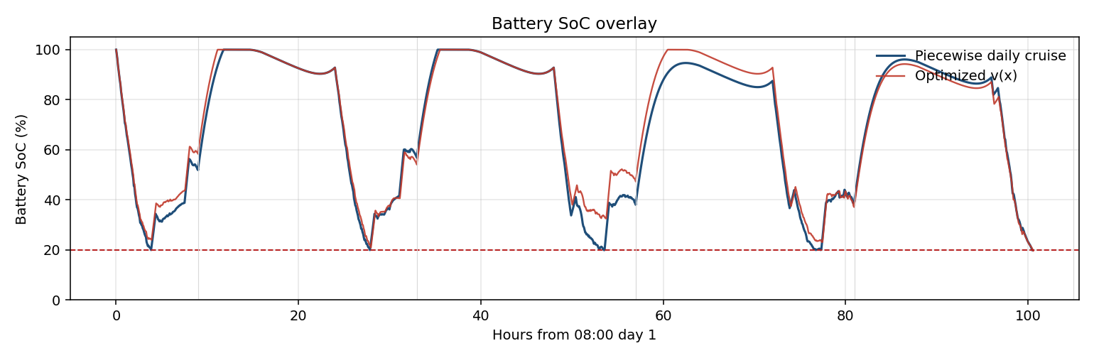
	Daily cruise	Optimized $v(x)$
Finish	3041 km, day 5	3041 km, day 5
Clock from 08:00 day 1	100.49 h	100.59 h
Moving time	35.99 h	36.09 h
Speeds	84.0, 82.1, 86.2, 85.3, 85.3 km/h	bins 80.4–87.8 km/h
Mean $|\Delta v|$	—	1.3 km/h

The freer profile finished about six minutes later, wiggling around the same ~85 km/h rail. That is the validation I wanted before treating Algorithm 1 as the strategy object below: support for the hypothesis, not a proof that no better policy exists.

---

Evaluation

After this work I keep two plants in my head.

The hopeful one is the theory baseline: $C_{DA} = 0.092$ (what was sitting in the inherited code), a fat Gaussian, 50 W hotel, still air. I use it to check that the planner behaves and to run one-knob tests.

The honest car is the same thing with $C_{DA} = 0.12$ — what coast-down / CFD said. That is the number I would actually plan on. I will get there.

Baseline — does the hopeful plant even look like a race?

Yes.

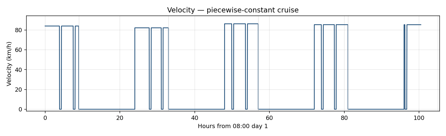
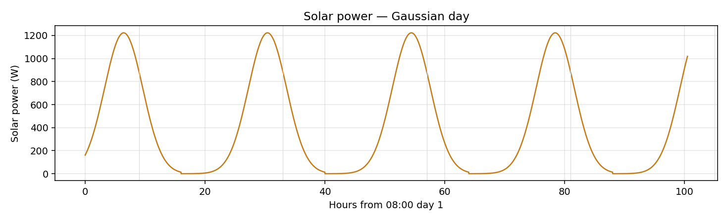
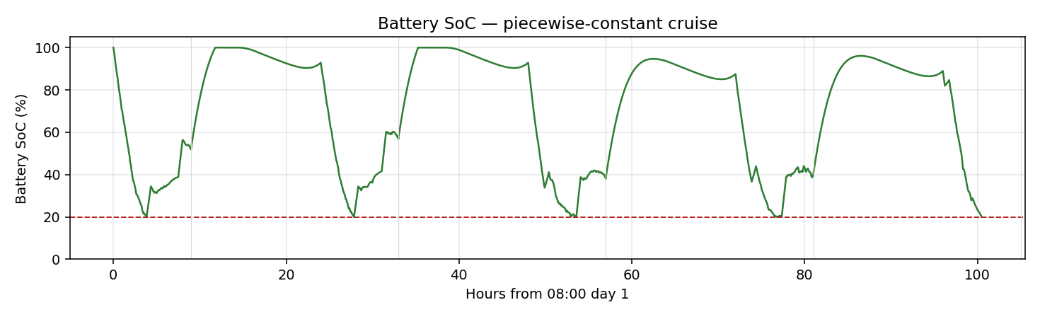
Five flat cruises (day-by-day 84.0, 82.1, 86.2, 85.3, 85.3 km/h), zeros at night and at control stops, SoC on the 20–100% rails. Adelaide on day 5, 3041 km, about 36.0 h moving, roughly 41.4 kWh from the array and 2.4 kWh from the pack, finishing on the 20% floor. SoC never invents energy; we empty at the line (on the draggy car later we will not — we sit in the sun longer and keep reserve).

This ~85 km/h number is not the race plan: the Gaussian is bright and $C_{DA} = 0.092$ is slipperier than the car we measured. It is the reference I kick.

Ablations — one knob, same planner

I keep Algorithm 1. I change one thing about the car or the world. Optimistic counterparts stay in the tables so you can see the other side of the knob; I just do not plan on them. A few rows are stress tests — physically possible, not a typical WSC week. I label those.

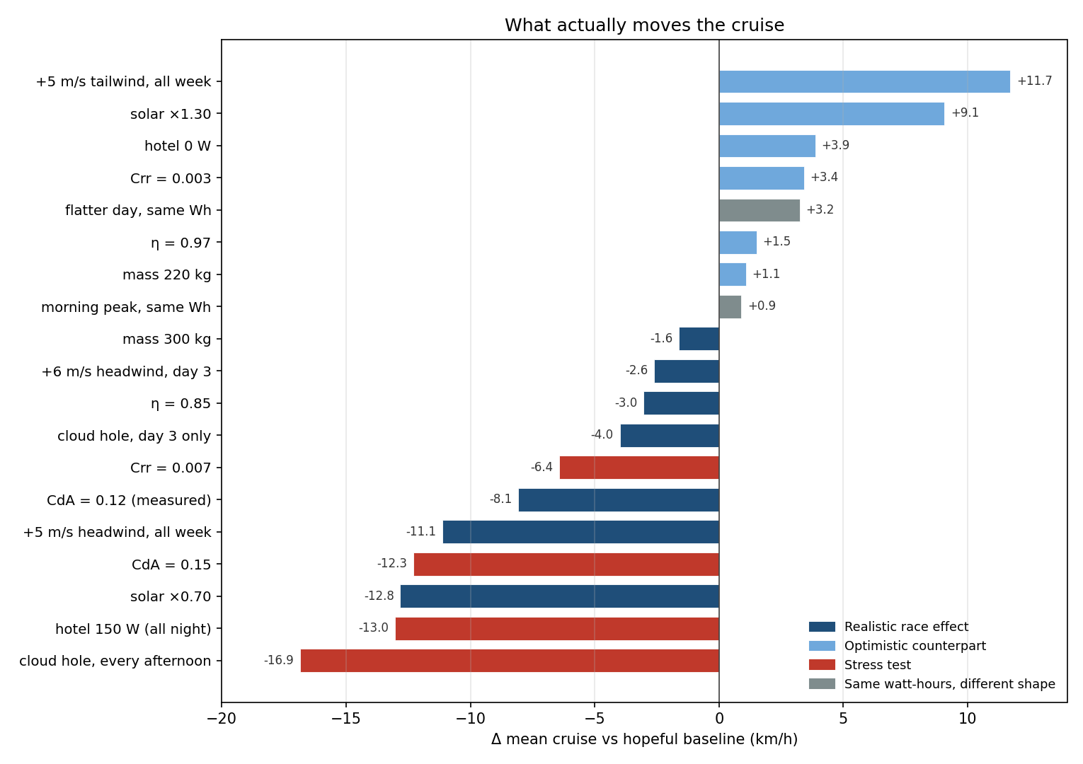
$\Delta$ is mean cruise versus the hopeful baseline (84.6 km/h). “Short” means we still drove most of the highway; 2743 km is about 300 km short, not 2700.

The car

Case	Mean cruise	$\Delta$	Distance	Finish?	Notes
$C_{DA} = 0.12$ (measured)	76.5	−8.1	3041 km	yes	Primary planning baseline.
$C_{DA} = 0.15$	72.3	−12.3	2972 km	no (~70 km short)	Dirty / yawed / vents open. Stress.
$C_{rr} = 0.003$	88.0	+3.4	3041 km	yes	Optimistic tire.
$C_{rr} = 0.007$	78.2	−6.4	3041 km	yes	Soft compound / pressure.
mass 220 kg	85.7	+1.1	3041 km	yes
mass 300 kg	83.0	−1.6	3041 km	yes	+40 kg ≈ 1.6 km/h.
$\eta = 0.85$	81.5	−3.0	3041 km	yes	Degraded drivetrain.
$\eta = 0.97$	86.1	+1.5	3041 km	yes	Optimistic.
hotel 0 W	88.5	+3.9	3041 km	yes	Lower bound.
hotel 150 W 24/7	71.5	−13.0	2893 km	no (~150 km short)	Continuous night drain. Stress.

The measured-drag run is the one I would radio.

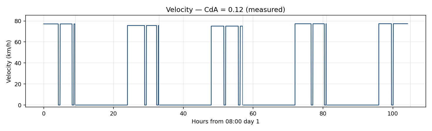
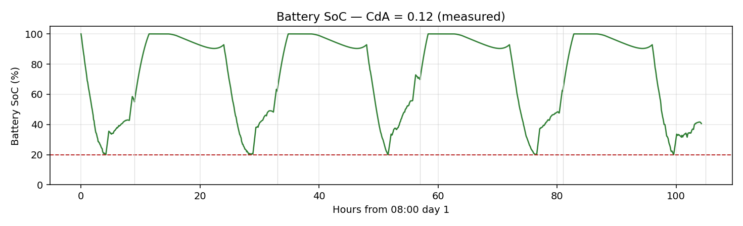
76.5 km/h, full 3041 km, day 5; daily holds in a 75–77 km/h band. Final SoC is ~41% because the planner holds the 20% floor each day and we arrive late with reserve — a finished race, not a missed one.

Mass is the quiet joke: +40 kg is 1.6 km/h; aero already owns the force balance. The other joke is hotel: 150 W × 15 h overnight is most of the pack before the sun. Daytime 50 W is a thin slice of cruise power; the lever is a night switch, not a 20 W daytime diet. The 150 W row is stress, not “LV rivals aero.”

The world

Case	Mean cruise	$\Delta$	Distance	Finish?	Notes
solar ×0.70	71.8	−12.8	2902 km	no (~140 km short)	Dim week / over-bright baseline.
solar ×1.30	93.7	+9.1	3041 km	yes	Brighter than an already bright curve.
flatter day, same Wh	87.8	+3.3	3041 km	yes	Shape change, energy fixed.
morning peak, same Wh	85.5	+0.9	3041 km	yes	Shape change, energy fixed.
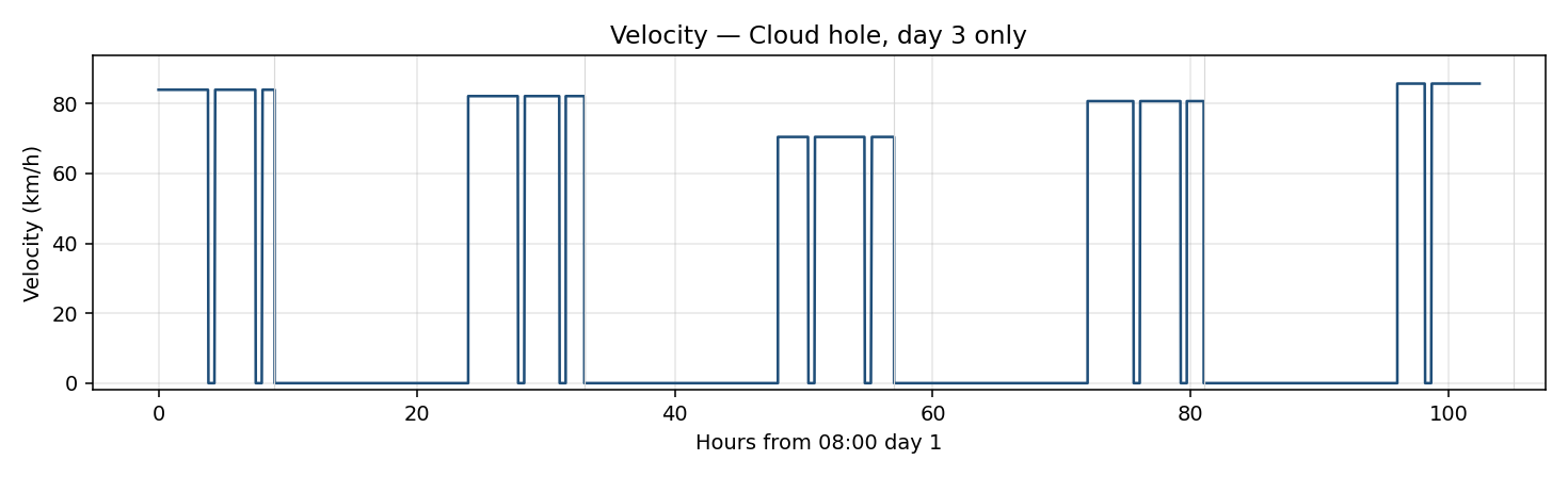
hole 13:00–16:00, day 3	80.6	−4.0	3041 km	yes	Single cloud band.
hole every afternoon	67.7	−16.9	2743 km	no (~300 km short)	Stress.
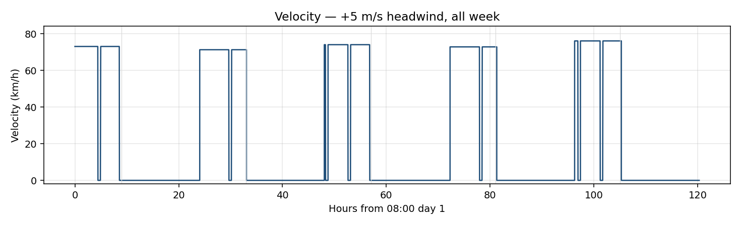
+5 m/s headwind, all week	73.5	−11.1	2994 km	no (~50 km short)	Harsh wind week.
+5 m/s tailwind, all week	96.3	+11.7	3041 km	yes	Favourable week.
+6 m/s headwind, day 3	82.0	−2.6	3041 km	yes	Single windy day.

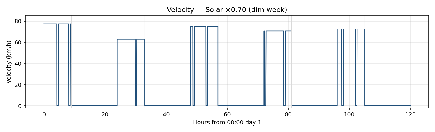
Watt-hours, not the hump. Same 06:00–18:00 energy with a flatter or morning-peaked shape moves cruise only 1–3 km/h; cut energy 30% and you are in DNF territory. Model daily irradiance energy; do not add a prettier sunrise.

One bad afternoon is not the week. A single 13:00–16:00 hole on day 3 costs ~4 km/h mean and a slower that day — you still finish. Every afternoon (~300 km short) is a stress test, not a claim about inland Australia.

Headwind is extra $C_{DA}$: +5 m/s all week ≈ 11 km/h; one windy day is a few km/h that day. The inherited model had no wind — an optimistic world.

Takeaways

I am not a chassis or array specialist; this is what the sensitivities suggest, not a build guide.

High leverage. Daily watt-hours (and an update when the forecast changes) matter more than sunrise shape — reshape at fixed energy barely moves cruise; cut ~30% and finish is at risk. Panel area is rule-capped, so the practical answer to a dimmer week is array efficiency and harvest (clean panels, mismatch, MPPT, shade when parked) and logging kWh into the pack, not only open-circuit voltage. Drag, including wind, ranks next: measured $C_{DA} = 0.12$ already costs ~8 km/h versus the hopeful 0.092, and 0.15 can fail here. Keeping the body clean looks worth more than shaving tens of kilograms; a coarse parallel wind belongs next to solar energy.

Medium. Rolling resistance is several km/h; drivetrain $\eta$ in the 0.85–0.97 band a few more — worth not running hot and messy, not a season rebuilt around a loss map. Hotel is a night story; daytime tens of watts are thin versus cruise power.

Low. Mass (+40 kg ≈ 1.6 km/h) and freer $v(x)$ / high-order plant detail did not change Tuesday morning’s speed in these tests. A simple plant — aero, rolling, mild grade, one $\eta$, hotel, sun/wind, watt-hour tank, race clock — was enough.

The loop that matches that ranking: today’s expected energy + today’s wind → today’s cruise.

---

Closing

I started this wanting a better optimiser. What I needed was a smaller question: the fastest legal cruise the pack and the sun will allow, one day at a time, without going through 20%.

The plant above is necessary where aero and daily solar energy move cruise by tens of km/h, and sufficient where freeing $v(x)$, reshaping the sun at fixed watt-hours, or adding motor temperature does not change the radio call. Hopeful plant ≈ 85 km/h; measured car ≈ 76 km/h; both day-5 finishes. That is enough for Tuesday morning on Agneya — not a forecast of Wednesday.

If you spot an error in the formulation or the tests, I would be glad to hear it.

All code to reproduce the model and the results can be found here- https://drive.google.com/file/d/1vD-gCd5PK4qKpSU1KzBC5WPY3KFAnwta/view?usp=sharing

References

1. P. G. Howlett, P. J. Pudney, T. Tarnopolskaya, and D. Gates, Optimal driving strategy for a solar car on a level road, IMA Journal of Mathematics Applied in Business and Industry, 8(1):59–81, 1997.
2. P. J. Pudney and P. G. Howlett, An optimal driving strategy for a solar powered car on an undulating road, Dynamics of Continuous, Discrete and Impulsive Systems, 4(4):553–567, 1998. (UniSA record)
3. P. J. Pudney and P. G. Howlett, Critical speed control of a solar car, Optimization and Engineering, 3:97–107, 2002.
4. P. J. Pudney and P. G. Howlett, An optimal battery interchange policy for a solar car, ANZIAM Journal.
5. E. Betancur, G. Osorio-Gómez, and others, Heuristic Optimization for the Energy Management and Race Strategy of a Solar Car, Sustainability, 9(10):1576, 2017. (survey of mathematical vs heuristic solar-car strategy)

---